For any non-product related queries, please write to info@perfios.com.
For any non-product related queries, please write to info@perfios.com.


In the previous article, we have introduced and discussed an opencv based solution to solve the Table Identification task. We have also discussed a few limitations that the rule based structure recognition methods have. We also gave some post-credits on using Graph Neural Networks for overcoming these limitations. To recall, let’s revisit the challenges before diving into the solution.
● Traditional computer vision methods (Hough lines, edge detections etc), that we use to detect lines, are always limited by the quality of the scan.
● For the semi-bordered tables, we have to use heuristics to mark row and column separators, and these heuristics have to be carefully chosen, which ultimately does not allow us to scale up whenever we onboard a new template of tables.
● An inherent limitation of the rule based approach, which identifies cells as row and column line intersections, is generation of multi-row or multi-column spanning cells.
Our ultimate goal is to identify each cell, its logical location (which row and column it belongs to). Can we do it by finding the adjacent cells? This definition allows us to treat each cell independently and cell sizes within the same row or same column can have various lengths (which is often seen for merged cells, comprising multiple rows or columns, as shown in Figure 1). These independent cells can be considered as independent nodes or vertices of a graph comprising the tabular content within the scanned document. Given these cells, we want to find the adjacency between these cells.
Let us understand this idea with figure 1. On the left, we have a sample table with a multi row spanned cell containing the word ‘TriStar’ and a multi-column spanned cell containing the word ‘Creek’. On the right, we have the same table but with the internal structural lines removed. Now if we consider each word as a node in the graph, say a graph with 10 nodes where nodes belong to the set {‘TriStar’, ‘Creek’, ‘Products’, ‘38’, ….}
The problem that we want to solve is, ‘for each pair of nodes (or pair of words in this table graph), are they adjacent to each other via row or column?’

Figure 1: A random table in the left half. On the right, we have the same table with internal structure removed.
We can also extend the problem to solve for cell adjacency, where we consider them adjacent if they reside in the same cell.
To elaborate on this idea of adjacency, let’s consider the same graph with some circles and lines added. The circles denote the position of nodes or words and the edges or lines represent the adjacency. Now consider the two observations about the nodes ‘investment’ and ‘TriStar’. In the figure Figure 2,
● The word ‘investment’ in the second row, first column, marked with green circle is row adjacent to the words {‘agencies’, ‘225.6’} also marked with green circles and are connected with the word investment with green lines (or edges). We can also see, the words ‘agencies’ and ‘225.6’ are themselves adjacent, so an edge is present between them.
● For the cell containing word ‘TriStar’, which spans two different rows, we can see that it is adjacent to {‘Creek’} as well as {‘Products’, 38’}. The blue lines denote the adjacency of ‘TriStart’ with ‘Creek’ and pink lines denote its adjacency with {‘Products’, ‘38’}. Again, as ‘Products’ and ‘38’ are adjacent among themselves, we do have one edge between them.
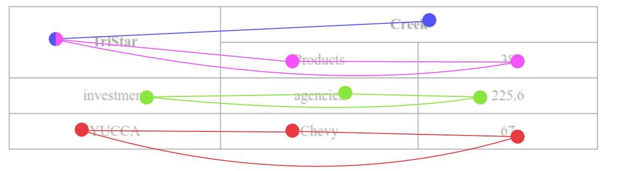
Figure 2: Table graph with coloured lines showing the adjacency according to table rows [Source: TIES:2.0]
Another way to define adjacency at a column level is shown in Figure 3. We can see that all the word pairs that are column adjacent have been connected with an edge.
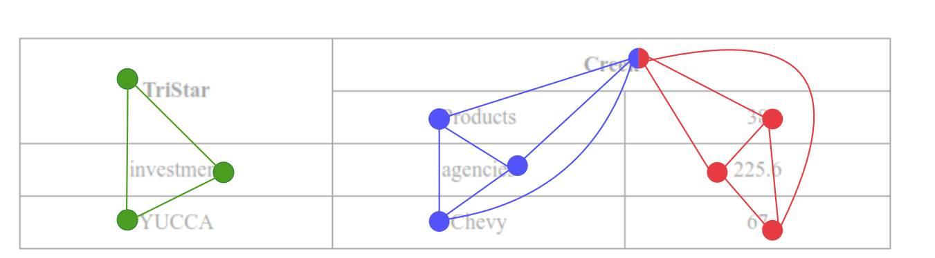
Figure 3: Table graph with coloured lines showing the adjacency according to table columns [Source: TIES:2.0]
Now the overall table structure identification has a slight modification of node classification problem. In a node classification problem, we classify each node into one of the predefined categories. In this task, as mentioned earlier, we are working on pairs of nodes and what we are classifying is if a pair of nodes is adjacent or not, i.e., a binary classification problem applied on a pair of nodes.
If we are familiar with cat vs dog classification (or cat vs NO cat classification, indirectly solving the same problem) using an artificial neural network, we can use a similar network to identify if two nodes are adjacent.
The only trick here is we have to capture some strong features about these nodes, that will enable the network to differentiate if the nodes are similar or dissimilar. We employ three neural networks to predict the adjacencies of each type viz, adjacent via rows, adjacent via columns and vis cells. All these networks will use the same strong features which we derive using the so called ‘Graph Neural Networks’.
Graph neural networks work on the principles of message passing. Based on our use case, we can apply different message passing flavors. Message passing is an iterative way to update the information. In our case, the features of each node get updates. At the end of one iteration, all of the nodes get their new features which (of course, if designed properly :P) are stronger than existing features. Researchers of TIES-2.0 have tried using an algorithm 'Dynamic Graph Convolutional Neural Networks’ for this message passing. But wait, what are these features at the start of the iteration?
Well, these features can be application specific. As the row and column spans are geometric features, choosing the coordinates of the words becomes a natural choice. Since we are working with financial statements, words like ‘NEFT’, ‘UPI’, ‘ATM’, ‘Credit’ have strong importance. So, we can also include some information (word embeddings) about the text in the node features. These two sets of information to create initial features is sufficient for the downstream task and can be easily fetched if we use OCR techniques. We can also feed in the CNN features, i. E., the visual information present at the node (at the crop of the image where the text is residing). Though these features will not be distinct enough for different nodes, tagging them along is worth a try. Well we have to use a convolutional neural network for getting these features. So far we have been talking about artificial neural networks, graph neural networks and now convolutional neural networks also. How are we going to fuse these together? Yes, with just the reverse order of their mentions.
Figure 4.1 and 4.2 summarize the entire architecture. We use the same table cropped image patch and feed it to OCR and Convolutional neural networks. OCR identifies the word text and the coordinates of the bounding box of the word. We can replace the text by its word embedding. Thus the word embedding with the word coordinates from one part of our node features. The CNN network(a shallow convolutional neural network) will extract the visual information of the image. We crop the visual features at each word location and combine it with respective word features. Thus visual features combined with word features form our node embeddings. In the figure, we have shown such node feature creations for the words ‘Creek’, ‘TriStar’ and ‘67’ with green, blue and orange colors respectively.
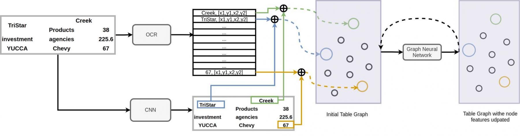
Fig. 4.1 : Network architecture - Part I
The word graph with initial node features is then iteratively processed with Graph neural network (DGCNN) in our case. At each iteration, the node features get updated.
We use pairs of nodes and pass them to three dense neural networks which will learn if the two nodes are adjacent or not with row-adjacency, column-adjacency or cell. Since the adjacent node pairs will be higher than non-adjacent nodes, we use a balanced sampling module(not shown in the figure to avoid complexity of the diagram) inspired from TIES:2.0’s monte carlo sampling. This sampling technique will generate an equal number of adjacent node pairs and non-adjacent node pairs, using the ground truth information that we pass. We also restrict the pairs to be selected within a radius of 6 hops. These are empirical numbers that work best so far for our task.
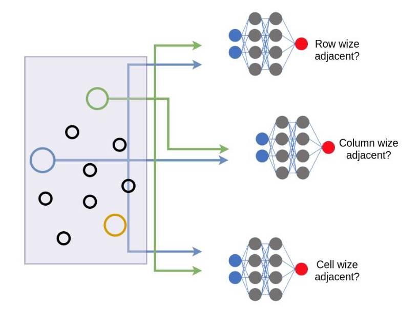
Fig. 4.2: Network Architecture-Part II
Let’s talk about training this complicated architecture.
To train this architecture faster, we store the OCR output offline as it will be static for each image throughout the training. So, each iteration starts with CNN forward propagation to get the visual features or CNN features. We concatenate it with word features to form the node features. Then we use monte carlo sampling that will generate a K number of pairs with a balance between adjacent node pairs and non-adjacent node pairs. These K pairs are then passed to row, column and cell adjacency detection networks. We compute three separate weighted cross entropy losses from the predicted adjacency values from each of the dense networks and the respective ground truth adjacency values. The overall loss is then propagated back through the dense nets, then to the graph neural networks and then to the CNN network.
For easier training, we can use initial layers of pretrained CNN as well, which are trained for extracting visual features from document images. This way, by freezing the CNN weights, we can train only graph neural networks and dense net parameters.
Let’s see some of our initial results. From figure 5, on the left, we see results for words belonging to the same column (column adjacent nodes). We mark a candidate word in orange. The words marked in green have been predicted as words in the same column. As we can see, the model has done a decent job in finding the adjacent column words.
For the image on the right, we show row-sharing words in green for the word marked in orange.
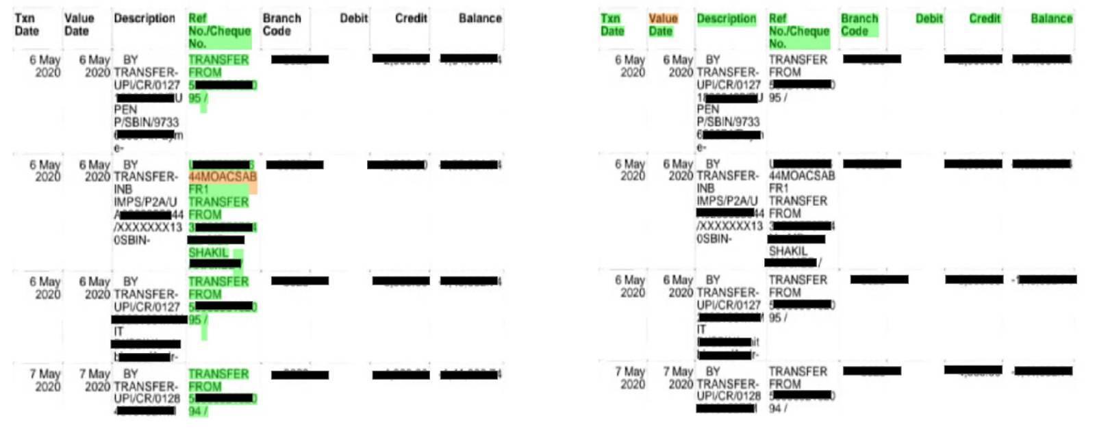
Figure 5: Initial results showing predicted adjacencies. On the left, the word colored in orange is the node under observation. The words predicted as column-adjacent are marked in green. Please ignore the words redacted in black color. On the right, we have the word ‘value’ colored in orange, for which row-adjacent words have been predicted and highlighted in green.
Of course, there are challenges that we are looking to solve. For example, in the following image (Figure 6), the word separation space within rows and across rows is uniform and the model predicts some extra words to be row-adjacent to the word marked in orange. But given that this is just scratching the surface for Table Structure Recognition using GNNs, it’s worth moving in the directions of GNNs.
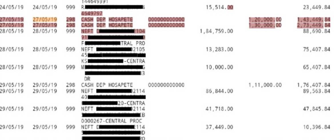
Figure 6: Results on table with uniform separation within and across rows. For the word colored in orange, the model predicts elements from its row as well as some elements from its previous and following rows also to be row-adjacent (colored in brown)
So, that’s all for this discussion, feel free to post your comments, queries or feedback. And thank you for spending your time reading this.